Sea Ice Viewer

This exemplary use case covers the creation of (a derivate of) the Sea Ice Viewer which has been part of AWI's Sea Ice Portal (meereisportal.de) for roughly a decade.

It covers the baseline (in terms of available data and motivation), the process of making the data available as map services following the according Standard Operating Procedures (SOP) and the creation and editing of the viewer frontend like described in the viewer user and creator manuals.

The backend tasks (data management, map service creation) will be described but not tangible for the reader. However, the resulting map services actually exist and their layers can be used to reproduce the viewer creation on your own (see the according chapter).

Baseline

You have sea ice concentration (SIC) data, derived from satellite measurements. They are on a daily basis, coming (most probably) in HDF files. You also used that data to calculate the monthly median edge of the sea ice. New data keeps coming!

Now you would like to make these data available als time series. To achieve this, you decide to create a Marine Data Viewer and start reading the docs 🤓.

Data Management

After reading the creator manual you figure out that your data needs to be hosted as a map service. You start with the SOPs, contact O2A Support and together you figure out the dataflows.

For the daily SIC, which is raster data, the O2A Support and you decide that GeoTIFF files – following the according O2A specification – are the best choice. For the monthly median edge, which is vector data, GeoCSV files – following the according O2A specification – should do the trick.

WARNING

The actual median edge dataflow uses shapefiles instead of GeoCSV files. However, that is a deprecated dataflow.

Using a project folder on AWI's Isilon network storage to exchange the data is agreed upon. You will place the initial files and new files on a daily (monthly) basis and AWI's Spatial Data Infrastructure (SDI) will check each morning for new data.

To generate the needed GeoTIFF and GeoCSV files you might want to use GDAL, for example within a cronjobbed Python script. However, this is totally up to you and beyond the scope of this document.

Map Service

After having set up the data flow, a representation of the (two) map services and the layers involved are created within the SDI's dataproduct configuration. For some (in this case historic) reason the decision is to place your dataproducts in two separate map services. There are some files to consider for you:

Sea Ice Dataproduct	Layer Folder	Layer Configuration Files
concentration	`platforms/satellite/gcomw1_amsr2_l2_sic`	platforms/satellite/gcomw1_amsr2_l2_sic/owner.layer.toml
median edge	`common/meereisportal/sea_ice_median_edge`	common/meereisportal/sea_ice_median_edge/owner.layer.toml

These files specify metadata for your layers. Title, abstract, keywords and both default and alternative styles (symbology) for the layers can be configured (by you!) here. For example, the concentration layer platforms/satellite/gcomw1_amsr2_l2_sic has the following metadata configured in its owner.layer.toml file and one of the referenced style files (sea_ice_concentration_2.sld). The following excerpts are shortened.

owner.layer.tomlsea_ice_concentration_2.sld

ini

# [...]

abstract = 'Sea Ice Concentration (coverage in %). Spatial Resolution: 3.125 km. Temporal Coverage: daily, since 2006. GCOMW1 AMSR2 passive microwave (acknowledgement to JAXA) processed by University of Bremen.'

keywords = [ "sea ice concentration", "satellite imagery", "remote sensing" ]

settings.style_default = "sea_ice_concentration_2"
settings.style_alternatives = [ "sea_ice_concentration" ]

# [...]

title = "Sea Ice Concentration (global)"

# [...]

xml

<!-- [...] -->

<sld:ColorMap>
    <sld:ColorMapEntry color="#f7fbff" label="   0.0 %" opacity="0.0" quantity="0"/>
    <sld:ColorMapEntry color="#deebf7" label="   6.5 %" opacity="0.2" quantity="6.5"/>
    <sld:ColorMapEntry color="#c7dcef" label="  13.0 %" opacity="0.5" quantity="13"/>
    <sld:ColorMapEntry color="#a2cbe2" label="  19.5 %" opacity="0.7" quantity="19.5"/>
    <sld:ColorMapEntry color="#72b2d7" label="  26.0 %" opacity="1.0" quantity="26"/>
    <sld:ColorMapEntry color="#4997c9" label="  32.5 %" opacity="1.0" quantity="32.5"/>
    <sld:ColorMapEntry color="#2878b8" label="  39.0 %" opacity="1.0" quantity="39"/>
    <sld:ColorMapEntry color="#0d57a1" label="  45.0 %" opacity="1.0" quantity="45"/>
    <sld:ColorMapEntry color="#000000" label="  50.0 %" opacity="1.0" quantity="50"/>
    <sld:ColorMapEntry color="#ffffff" label=" 100.0 %" opacity="1.0" quantity="100"/>
</sld:ColorMap>

<!-- [...] -->

In the background, SDI automation silently takes care of these information being processed, resulting in layers ready to use:

Sea Ice Dataproduct	WMS	Layer Name	Base + Capabilities URLs
concentration	`platforms/satellite`	`gcomw1_amsr2_l2_sic_4326`	`https://maps.awi.de/services/platforms/satellite/ows`, https://maps.awi.de/services/platforms/satellite/ows?REQUEST=GetCapabilities&SERVICE=WMS&VERSION=1.3.0
median edge	`common/meereisportal`	`sea_ice_median_edge`	`https://maps.awi.de/services/common/meereisportal/ows`, https://maps.awi.de/services/common/meereisportal/ows?REQUEST=GetCapabilities&SERVICE=WMS&VERSION=1.3.0

Viewer Configuration

To start with an empty viewer, go to a portal's viewers overview page (e.g. marine-data.de/viewers) and use the prominent CREATE YOUR OWN VIEWER! tile (screenshot) or directly visit the portal's new-viewer URL (e.g. marine-data.de/viewers/new).

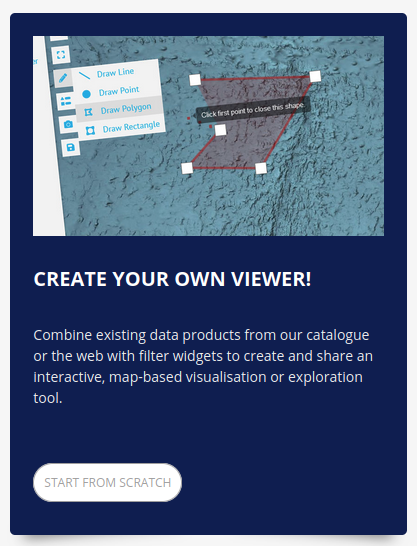
Select START FROM SCRATCH

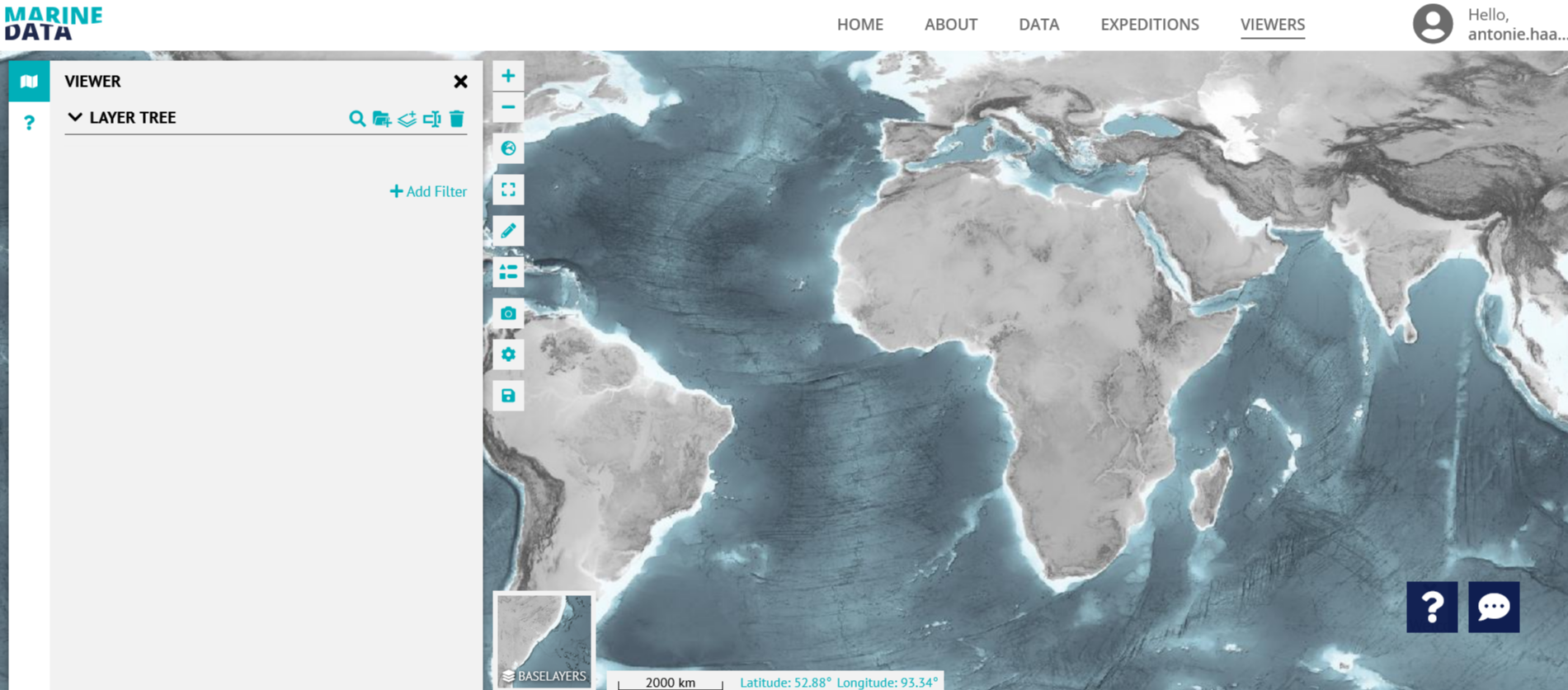
An empty viewer opens:

There are three steps to proceed:

Select the data
Configure the filter settings
Add the metadata

The order is not really relevant, but metadata does depend on data as well as filter settings.

Data

To add data: Open the DATA IMPORTER and enter sea ice in the search line:

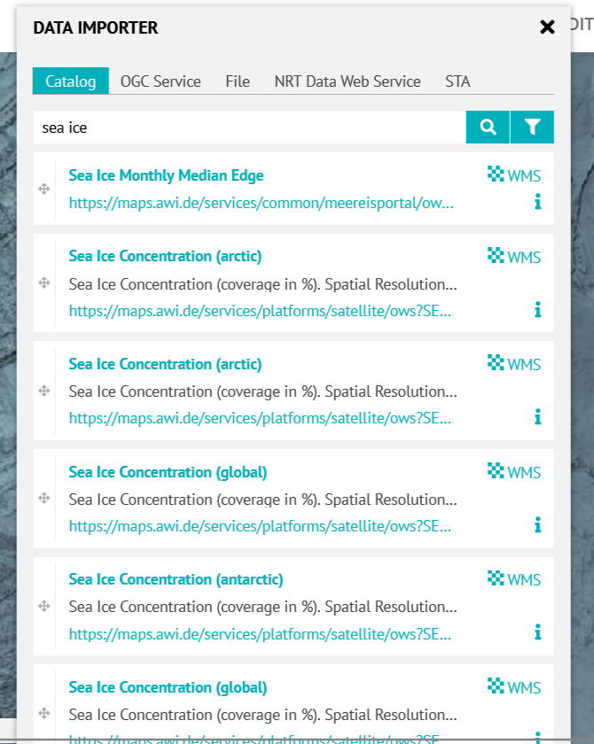
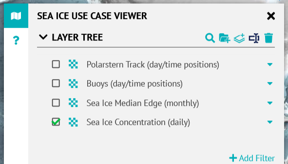
From the list select:

Sea Ice Monthly Median Edge
Sea Ice Concentration (global) for world view.

Important: If the (global) version is selected polar views (North and South) are possible. If (arctic) or (antarctic) view is selected it is just for the selected view, either Arctic or Antarctic.

Add additonally buoys and Polarstern tracks:

Before continuing: SAVE! To do this the name of the viewer has to be defined in the overview window that opens when the save button was used.

And don't forget to Save after adding the viewer name.

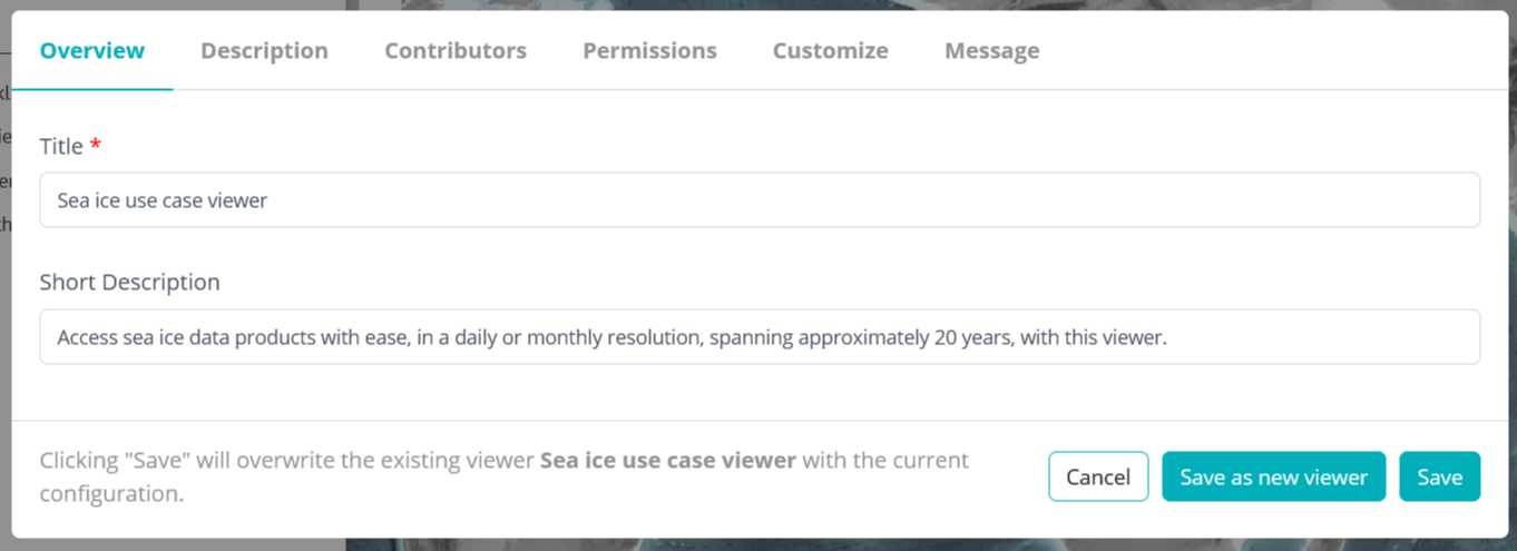
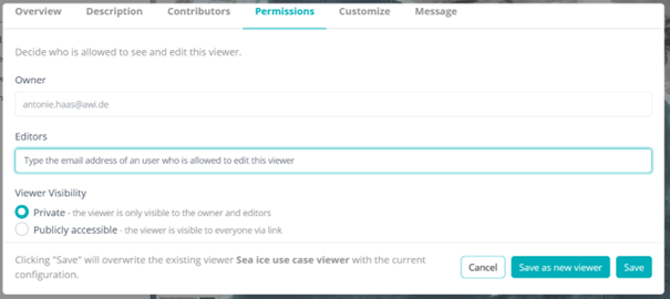
If others should be involved in the configuration or editing of this viewer, go to the 'Permissions' tab and enter their email addresses.

Anything changed? SAVE

Let's go back to the first step of configuring the data and filters. This is because the metadata and citations depend on the data. Therefore, it makes sense to finalise all the metadata and additional information after completing the data and filter steps.

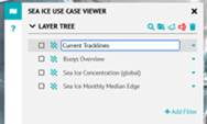
Select the 'Rename' option (shown in red) and click on the layer that you want to rename. Enter a name that highlights or specifies the data in this layer more precisely, e.g. add units or temporal resolutions.

If the listed layer should be moved to another position, hover over. The cursor changes to a hand an the layers can grabbed and moved to the new position. Generally, layers with small spatial extent shloud be placed on top and layers with high spatial extent on the beneath.

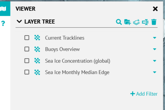
The new configuration of the Layer Tree might look like this:

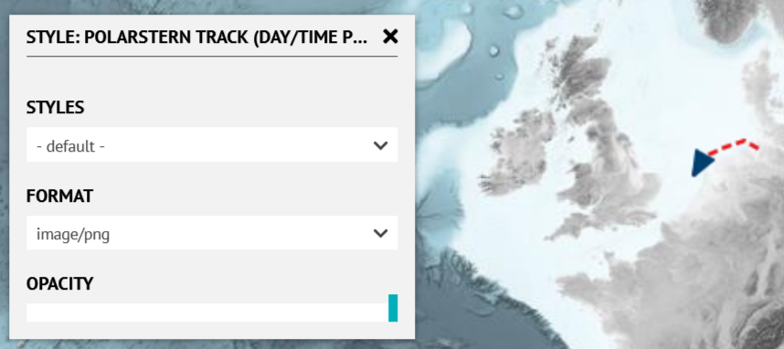
The layers come with default styles. However, there are other styles that can be applied using the Style menu, which opens when you click on the downward-facing triangle next to the layer title.

Filters

Once the data layers have been styled, the next step is to configure the filter settings. There are several filter widgets, but time is not only very exciting, it is also one of the most important variables for understanding scientific processes.

Two time filter widgets can be added here: one with daily temporal resolution and one with monthly temporal resolution.

Go to +AddFilter and select Temporal Filter.

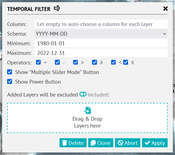
Rename the filter widget by clicking on the small icon next to the headline, which will turn red, and enter a meaningful name. Adjust all the other filter settings as shown in the screenshot.

INFO

Technical support is needed to tailor a temporal filter widget to raster-based WMS layers. Contact the O2A Support (o2a-support@awi.de).

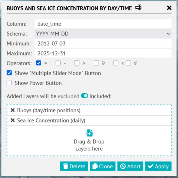
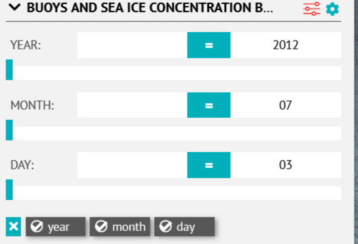
Select 'Advanced Settings' by tapping on the three lines between the filter name and the gear icon (it turns red). Additional filter settings, such as month or day, can now be activated and added to the displayed filter.

Add an addtional temporal filter that will be applied to the monthly median edge data layer.

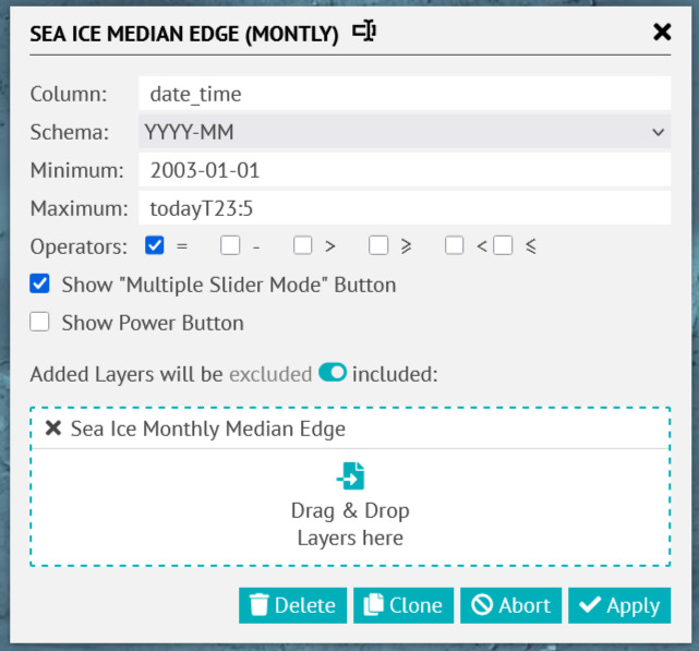
Again, the additional slider can be added by selecting Advanced Settings.

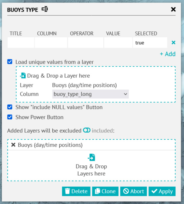
To filter by buoy type, add a checkbox filter. The configuration can be done on different ways. If the data layer is unkown Load Unique values is an option:

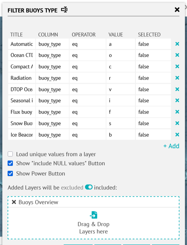
If the data table and its content is well-known the filter can be configured more individual as shown in this expamle:

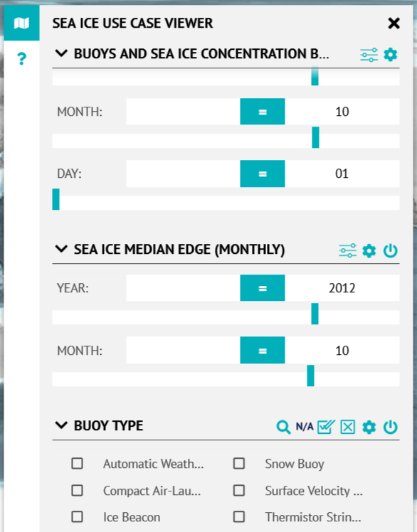
After adding all filter widgets all of them are listed in the Layer Tree.

As nothing will be saved automatically, it is important to save regularly.

SAVE!

Metadata

The final step to proceed is to add or complete the metadata. The instructions on how to do this can be found here: creator manual.

Example Use Cases

Guides

Specs

Sea Ice Viewer

Baseline